Working with notebooks
While working on a research project, Jupyter notebooks can be useful for prototyping and data exploration. If while working interactively in a notebook you get an output you like, e.g., a figure, it can be tempting to simply stop right there and copy/paste it into a research article. However, in order to keep the project reproducible, we need to be able to go from raw data to research article with a single command, which of course is not possible in the above scenario.
This is the primary notebook use case Calkit is concerned with: generating evidence to back up conclusions or answers to research questions. There are other use cases that are out of scope like using notebooks to build documentation or interactive web apps for exploring results. For building apps (a different concept in a Calkit project), there are probably better tools out there, e.g., marimo, Dash, Voila, or Gradio.
Here we'll talk about how to take advantage of the interactive nature of Jupyter notebooks while incorporating them into a reproducible workflow, avoiding some of the pitfalls that have caused a bit of a notebook reproducibility crisis. Returning to the "one project, one command" requirement, we can focus on three rules:
- The notebook must be kept in version control.
This happens naturally since any file included in a Calkit project is
kept in version control.
However, it's usually a good idea to exclude notebook output from
Git commits.
This can be done by installing
nbstripoutand runningnbstripout --installin the project directory. - A notebook must run in one of the project's environments.
- Notebooks should be incorporated into the project's
pipeline.
It's fine to do some ad hoc work interactively to get the notebook
working properly, but
"official" outputs should be generated by calling
calkit run. This means notebooks need to be able to run from top-to-bottom with no manual intervention. We'll see how below.
If you use JupyterLab, check out the Calkit JupyterLab extension docs.
Creating an environment for a notebook
Assuming you want to run Python in the notebook, you can create an environment
for it with uv, venv, conda, or pixi.
For example, if we wanted to create a new uv-venv called py in our project,
we can execute:
calkit new uv-venv \
    --name py \
    --prefix .venv \
    --python 3.13 \
    --path requirements.txt \
    jupyter \
    "pandas>=2" \
    numpy \
    plotly \
    matplotlib \
    polars
You can then start JupyterLab in this environment with
calkit xenv -n py jupyter lab.
Note the environment only needs to be created once per project. If the project is cloned onto a new machine, the environment does not need to be recreated, since that will be done automatically when the project is run. Also note that it's totally fine and perhaps even preferable to create a new environment for each notebook, so long as they have different names, prefixes, and paths---there is no limit to the number of environments a project can use, and they can be of any type.
Adding a notebook to the pipeline
A notebook can be added to the pipeline either with
calkit new jupyter-notebook-stage or
by editing the project's calkit.yaml
file directly.
For example:
# In calkit.yaml
environments:
  py:
    kind: uv-venv
    prefix: .venv
    python: "3.13"
    path: requirements.txt
pipeline:
  stages:
    my-notebook:
      kind: jupyter-notebook
      environment: py
      notebook_path: notebooks/get-data.ipynb
      inputs:
        - config/my-params.json
      outputs:
        - data/raw/data.csv
      html_storage: dvc
      executed_ipynb_storage: null
      cleaned_ipynb_storage: git
# Optional: Add to project notebooks so they can be viewed on Calkit Cloud
notebooks:
  - path: notebooks/get-data.ipynb
    title: Get data
    stage: my-notebook
For this example, we're declaring that the notebook
should use the py environment, and that it will read an input
file config/my-params.json and produce an output
file data/raw/data.csv.
These inputs and outputs will be tracked
along with the notebook and environment content,
to automatically determine if and when the notebook needs to be rerun.
Outputs will also be kept in DVC by default so others can pull them down
without bloating the Git repo.
Output storage is configurable, however, e.g., if you'd like to keep
smaller and/or text-based outputs in Git for simplicity's sake.
Copies of the notebook with and without outputs will be generated as the
notebook is executed, along with an HTML export of the latter.
Storage for these outputs can be controlled with the html_storage,
executed_ipynb_storage, cleaned_ipynb_storage properties,
and they will live inside the project's .calkit subdirectory.
The executed .ipynb can be rendered on GitHub or
nbviewer.org,
and the HTML can be viewed on calkit.io,
the latter of which allows some level of interactivity, e.g., Plotly figures.
The cleaned .ipynb can be useful for diffing with Git in cases where
nbstripout is not activated.
It's also possible to add a notebook to the pipeline
inside a notebook with the declare_notebook function,
which will update calkit.yaml automatically.
import calkit

calkit.declare_notebook(
    path="notebooks/get-data.ipynb",
    stage_name="my-notebook",
    environment_name="py",
    inputs=["config/my-params.json"],
    outputs=["data/raw/data.csv"],
    html_storage="dvc",
    executed_ipynb_storage=None,
    cleaned_ipynb_storage="git",
)
Note that for this to run properly calkit-python must be installed in
the notebook's environment, which in this case is named py and whose
packages are listed in requirements.txt.
If we didn't include them when creating the environment,
we can simply add calkit-python to the requirements.txt file and rerun
calkit xenv -n py jupyter lab.
The environment will be updated before starting JupyterLab.
Working interactively
The main advantage of Jupyter notebooks is the ability to work interactively, allowing us to quickly iterate on a smaller chunk of the process while the rest remains constant. For example, if you need to refine a figure, you can keep updating and running the cell that generates the figure, without needing to rerun the expensive cell above that generates or processes the data for it. In this case our notebook might look like this:
So, with a fresh Jupyter kernel we'll need to run cell 1 in order to generate
result so we can iterate on cell 2 to get the plot looking the way
we want it to.
But what if run_data_processing
takes minutes, hours, or even days, so therefore we don't want to run it
every time we restart the notebook?
Well, we can use the Calkit %%stage cell magic to automatically cache
and retrieve the result.
After adding a cell with:
the first cell can be turned into a pipeline stage by changing it to:
%%stage --name run-nb-proc --environment py --out result
from some_package import run_data_processing

result = run_data_processing(param1=55)
In the magic command we're giving the cell a unique name,
declaring which environment it should run in
(py above, but it can be any environment in the project),
and declaring an output from the cell that we want to be available to
cells below.
Now, the kernel can be restarted and we can use "run all cells above"
when working on the figure,
and we'll have result nearly instantaneously.
result will also be versioned with DVC and pushed to the cloud by default,
so our collaborators can also take advantage of the caching
without bloating the Git repo.
Execution as part of the project's pipeline will also take advantage of
the caching and will not rerun data processing unless something
about that cell's code or environment has changed.
For a more in-depth look at using the %%stage cell magic,
see this tutorial.
Parameterizing notebooks
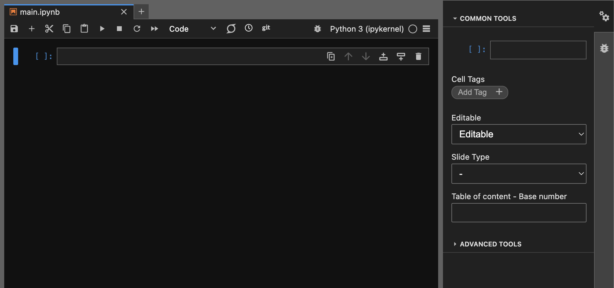
Thanks to Papermill, Calkit can run notebooks that have been parameterized, and executed versions will be saved with parameters in their names. To parameterize a notebook, first add a cell with the "parameters" tag and add your parameters there as variable declarations, e.g.,
In JupyterLab, you can use the property inspector to edit cell tags:
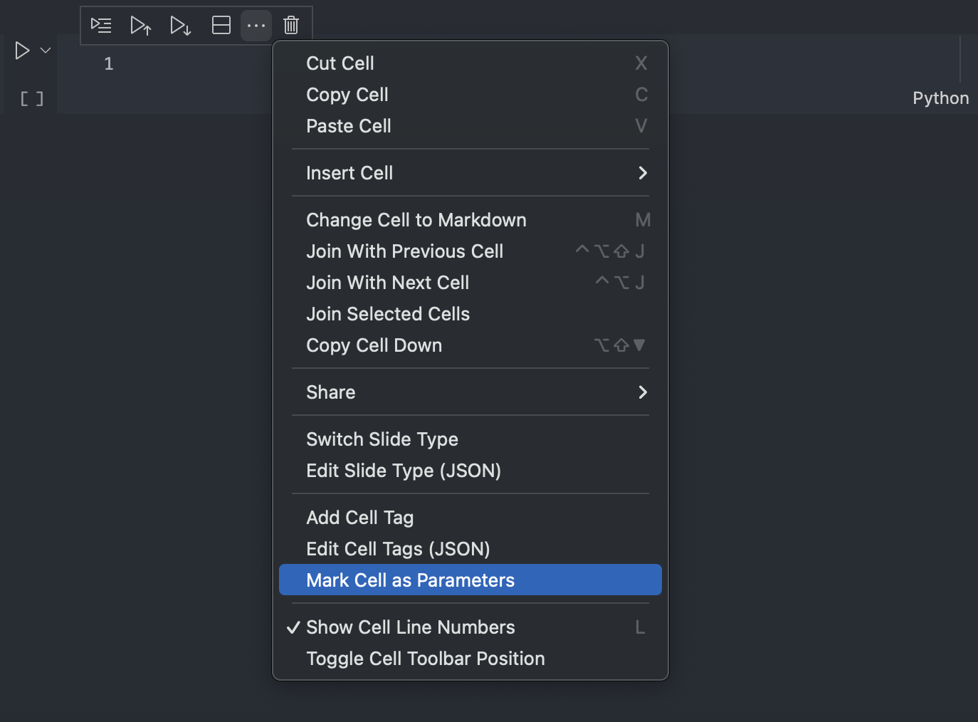
In VS Code, the cell context menu can be used to mark the cell as parameters:
Then, in the Calkit pipeline, add parameters to the notebook stage:
# In calkit.yaml
environments:
  main:
    kind: uv-venv
    path: requirements.txt
    prefix: .venv
    python: "3.13"
pipeline:
  stages:
    notebook-56-a:
      kind: jupyter-notebook
      notebook_path: notebook.ipynb
      environment: main
      parameters:
        param1: 56
        param2: a
    notebook-58-b:
      kind: jupyter-notebook
      notebook_path: notebook.ipynb
      environment: main
      parameters:
        param1: 58
        param2: b
Iterating over parameterized notebooks
The example below shows project-level parameters used to iterate over a notebook stage:
parameters:
  param1:
    - range:
        start: 0
        stop: 10
        step: 2
  param2:
    - random-forest
    - lightgbm
pipeline:
  stages:
    my-notebook-with-params:
      kind: jupyter-notebook
      environment: my-env
      notebook_path: notebook.ipynb
      iterate_over:
        - arg_name: param1
          values:
            - parameter: param1 # Args and params can be named differently
        - arg_name: param2
          values:
            - parameter: param2
      parameters:
        param1: "{param1}" # Notebook params can also be named differently
        param2: "{param2}"
      outputs:
        - results/param1={param1}/param2={param2}/results.csv
For more information, see pipeline iteration.